10 Gravitational Waves from Compact Binaries with White-Dwarf Components
We need to start this section with a caveat that until now virtually all studies on the detection of low-frequency GWR from compact binaries, with the single exception of [531*], have been made with the future launch of LISA in mind. At the time of writing only several months have elapsed since the decision to cancel LISA and the introduction of the eLISA project. Therefore, almost all estimates involving sensitivity of the detector are still “LISA-oriented” and only in some cases corrections for the reduced (by about an order of magnitude) eLISA sensitivity are available. Nevertheless, as the physics behind GWR emission is unchanged, we present in this section, as examples, “LISA-oriented” results, unless stated otherwise.It was suggested initially that contact W UMa binaries will dominate the Galactic gravitational-wave background at low frequencies [487]. However, it was shown in [784, 467, 180*, 426*, 282*] that it will, most probably, be totally dominated by detached and semidetached WD binaries.
As soon as it was recognized that the birth rate of Galactic close WD binaries may be rather high, and
even before detection of the first close detached DD was reported in 1988 [665], in 1987 Evans, Iben, and
Smarr [180] accomplished an analytical study of the detectability of the signal from the Galactic ensemble
of DDs, assuming certain average parameters for DDs. Their main findings can be formulated as follows. Let
us assume that there exists a certain distribution of DDs over frequency of the signal  and the
strain amplitude
and the
strain amplitude  :
:  . The weakest signal is
  . For the time span of observations
 , the frequency resolution bin of the detector is
  . Then, integration of
 over amplitude down to a certain limiting
  and over
  gives the mean number of
sources per unit frequency resolution bin for a volume defined by
gives the mean number of
sources per unit frequency resolution bin for a volume defined by  . If for a certain

 overlap. If in a certain resolution bin
  does not exist,
individual sources may be resolved in this bin for a given integration time (if they are above the detector’s
noise level). In the bins where binaries overlap, they produce “confusion noise”: an incoherent sum of
signals; the frequency above which the resolution of individual sources becomes possible was referred to as
the “confusion limit”,
does not exist,
individual sources may be resolved in this bin for a given integration time (if they are above the detector’s
noise level). In the bins where binaries overlap, they produce “confusion noise”: an incoherent sum of
signals; the frequency above which the resolution of individual sources becomes possible was referred to as
the “confusion limit”,  . Evans et al. found
  and
and  for integration times 106 s
and 108 s, respectively.
for integration times 106 s
and 108 s, respectively.
Independently, the effect of confusion of Galactic binaries was demonstrated by Lipunov, Postnov, and Prokhorov [427], who used simple analytical estimates of the GW confusion limited signal produced by unresolved binaries whose evolution is driven by GWs only; in this approximation, the expected level of the signal depends solely on the Galactic merger rate of WD binaries (see [252*] for more details). Later, analytic studies of the GW signal produced by stellar binaries at low frequencies were continued in [187, 282, 608, 281*]. A more detailed approach to the estimate of the GW foreground is possible using population synthesis models [426, 828*, 518*, 519*, 661, 864*, 865*]. Convenient analytical expressions allowing us to compare the results of different studies as a function of the assumed Galactic model and merger rate of dwarf binaries are provided by Nissanke et al. [531*].
Note that in early studies the combined signal of Galactic binaries was dubbed “background” and considered as a “noise”. However, Farmer and Phinney [188] stressed that this signal will in fact be a “foreground” for “backgrounds” produced in the early universe. But only circa 2008 – 2009 the term “foreground” became common in discussions of Galactic binaries. As summarized by Amaro-Seoane et al. [10], the overall level of the foreground is a measure of the total number of ultra-compact binaries; the spectral shape of the foreground contains information about the homogeneity of the sample, as models with specific types of binaries predict a very distinct shape; the geometrical distribution of the sources can be found by a probe like eLISA.
Giampieri and Polnarev [240], Farmer and Phinney [188] and Edlund et al. [170*] showed that, due to the concentration of sources in the Galactic center and the inhomogeneity of the LISA-antenna pattern, the foreground should be strongly modulated in a year of observations (Figure 29*), with time periods in which the foreground is by more than a factor two lower than during other periods. This is not the case for the signal from extra-galactic binaries, which should be almost isotropic. The characteristics of the modulation can provide information on the distribution of the sources in the Galaxy, as the different Galactic components (thin disk, thick disk, halo) contribute differently to the modulation. Additionally, during “low signal” periods, antenna will be able to observe objects that are away from the Galactic plane.
Referring the reader for comprehensive review of eLISA science to [10], we briefly note that measurements of individual binaries provide the following information. If the system is detached, the evolution of the signal is dominated by gravitational radiation and, in principle, three variables may be measured:
where
 is the strain amplitude,
  is the frequency,
  is the chirp mass,
and
is the chirp mass,
and  is the distance to the source. Thus, the determination of
  ,
,  , and
, and  (which is expected to
be possible for 25% of eLISA sources [10]) provides
(which is expected to
be possible for 25% of eLISA sources [10]) provides  and
and  . The value of
  (which may be
possible for a few high-SNR systems) gives information on deviations from the “pure” GW
signal due to tidal effects and mass-transfer interactions. An estimate of the effects of tidal
interaction is especially interesting, since it is expected that this effect will be typical for pre-merger
systems in which it may lead to strong heating, raising the luminosity of each component to
(which may be
possible for a few high-SNR systems) gives information on deviations from the “pure” GW
signal due to tidal effects and mass-transfer interactions. An estimate of the effects of tidal
interaction is especially interesting, since it is expected that this effect will be typical for pre-merger
systems in which it may lead to strong heating, raising the luminosity of each component to
 , which gives a chance of optical detection on the time scale of a human life; moreover,
it can even affect conditions for thermonuclear burning in the inner and outer layers of WD
[829, 304, 827, 218, 219].
, which gives a chance of optical detection on the time scale of a human life; moreover,
it can even affect conditions for thermonuclear burning in the inner and outer layers of WD
[829, 304, 827, 218, 219].
Nelemans et al. [518*] constructed a population synthesis model of the gravitational-wave signal from the Galactic disk population of binaries containing two compact objects. The model included detached DDs, semidetached DDs,32 detached systems of NSs and BHs with WD companions, NS and BH binaries. For details of the model we refer the reader to the original paper and references therein. Table 8 shows a number of systems with different combinations of components in the Nelemans et al. model.33 Note that these numbers strongly depend on assumptions in the population synthesis code, especially on the normalization of the stellar birth rate, star formation history, distributions of binaries over initial masses of components, their mass-ratios and orbital separations, the treatment of stellar evolution, common envelope formalism, etc. For binaries with relativistic components (i.e., descending from massive stars) an additional uncertainty is brought in by assumptions on stellar wind mass loss and natal kicks. The factor of uncertainty in the estimated number of systems of a specific type may easily exceed 10 (cf. [265, 518*, 791, 294, 519*, 661, 864*]). Thus, these numbers should be taken with some caution.
Table 8 immediately shows that detached DDs, as expected, dominate the population of compact
binaries, as found by other authors, as well. While Table 8 gives total numbers, examples of contributions
from different formation channels and spatial components of the Galaxy may be found, e.g.,
in [661, 864*, 865], with a caveat that models in these paper are different from the model in [518*].
Population-synthesis studies confirmed the expectation that a contribution to the signal in the LISA/eLISA
frequency range from thick disk, halo, and bulge binaries should not be significant, since the
binary systems there are predominantly old and either merged or evolved to too long periods
as IDD [660, 864*, 661]. It was also shown that the contribution from extra-galactic binaries
to the signal in the LISA/eLISA range will be  1% of the foreground [188]. The list of
models computed before 2012 and an algorithm allowing one to compare the results of different
calculations to the extent of their dependence on Galactic model and normalization may be found
in [531*].
1% of the foreground [188]. The list of
models computed before 2012 and an algorithm allowing one to compare the results of different
calculations to the extent of their dependence on Galactic model and normalization may be found
in [531*].
Population synthesis computations yield the ensemble of Galactic binaries at a given epoch with their
specific parameters  ,
,  , and
, and  and the Galactic location. Figure 30* shows examples of
the relationship between the frequency of emitted radiation and amplitude of the signals from
the “typical” double degenerate system that evolves into contact and merges, for an initially
detached double degenerate system that stably exchanges matter after the contact, i.e., an
AM CVn-type star and its progenitor, and for an UCXB and its progenitor. For the AM CVn
system effective spin-orbital coupling is assumed [512, 464*], Figure 22*. The difference in the
properties and evolution of DD and IDD (merger vs. bounce and continuation of evolution with
decreasing mass) is reflected in the distributions and magnitude of their strains shown in Figure 31*
[170*].
and the Galactic location. Figure 30* shows examples of
the relationship between the frequency of emitted radiation and amplitude of the signals from
the “typical” double degenerate system that evolves into contact and merges, for an initially
detached double degenerate system that stably exchanges matter after the contact, i.e., an
AM CVn-type star and its progenitor, and for an UCXB and its progenitor. For the AM CVn
system effective spin-orbital coupling is assumed [512, 464*], Figure 22*. The difference in the
properties and evolution of DD and IDD (merger vs. bounce and continuation of evolution with
decreasing mass) is reflected in the distributions and magnitude of their strains shown in Figure 31*
[170*].
Note that there is a peculiar difference between WD pairs that merge and pairs that experience a stable
mass exchange. The pairs that coalesce stop emitting GWs on a relatively short time-scale (on the order of
the period of the last stable orbit, typically a few minutes) [443]. Thus, if we would be lucky to observe a
chirping WD and a sudden disappearance of the signal, this will manifest a merger. However, the chance to
detect such an event is small since the Galactic rate of merging WD binaries is  only.
only.
For the system with a NS, the mass exchange rate is limited by the critical Eddington value, and excess
of matter is “re-ejected” from the system (see Section 3.3.3 and [877]). Note that for an AM CVn-type star
it takes only  300 Myr after contact to evolve to
  , which explains their accumulation at
lower
, which explains their accumulation at
lower  . For UCXBs this time interval is only
  20 Myr.
| Type | Birth rate | Merger rate | Number |
| Detached DD | 2.5 × 10⁻² | 1.1 × 10⁻² | 1.1 × 10⁸ |
| Semidetached DD | 3.3 × 10⁻³ | — | 4.2 × 10⁷ |
| NS + WD | 2.4 × 10⁻⁴ | 1.4 × 10⁻⁴ | 2.2 × 10⁶ |
| NS + NS | 5.7 × 10⁻⁵ | 2.4 × 10⁻⁵ | 7.5 × 10⁵ |
| BH + WD | 8.2 × 10⁻⁵ | 1.9 × 10⁻⁶ | 1.4 × 10⁶ |
| BH + NS | 2.6 × 10⁻⁵ | 2.9 × 10⁻⁶ | 4.7 × 10⁵ |
| BH + BH | 1.6 × 10⁻⁴ | — | 2.8 × 10⁶ |
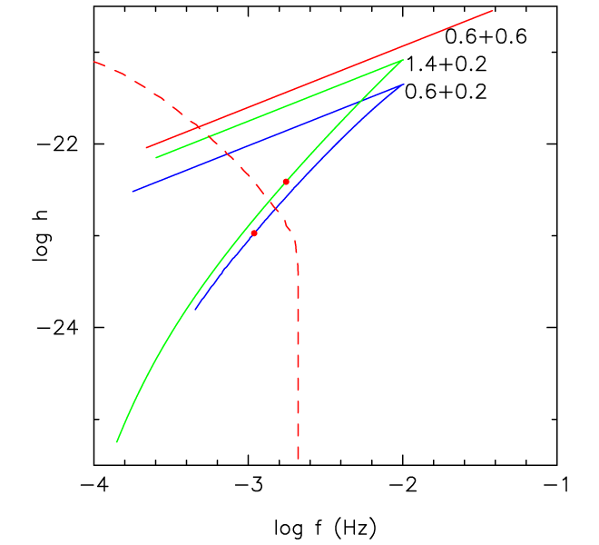
 (red line), a WD + WD system with
 (blue line) and a NS + WD system with
  (green line). All
systems have an initial separation of components
(green line). All
systems have an initial separation of components  and are assumed to be at a distance of
1 Kpc (i.e., the actual strength of the signal has to be scaled with factor
and are assumed to be at a distance of
1 Kpc (i.e., the actual strength of the signal has to be scaled with factor  , with
  in Kpc).
For the DD system, the line shows an evolution into contact, while for the other two systems the
upper branches show pre-contact evolution and lower branches – a post-contact evolution with mass
exchange. The total time-span of evolution covered by the tracks is 13.5 Gyr. Red dots mark the
positions of systems with components’ mass ratio
in Kpc).
For the DD system, the line shows an evolution into contact, while for the other two systems the
upper branches show pre-contact evolution and lower branches – a post-contact evolution with mass
exchange. The total time-span of evolution covered by the tracks is 13.5 Gyr. Red dots mark the
positions of systems with components’ mass ratio  , below which the conventional picture
of evolution with a mass exchange may be not valid. The red dashed line marks the position of the
confusion limit as determined in [519*].
, below which the conventional picture
of evolution with a mass exchange may be not valid. The red dashed line marks the position of the
confusion limit as determined in [519*].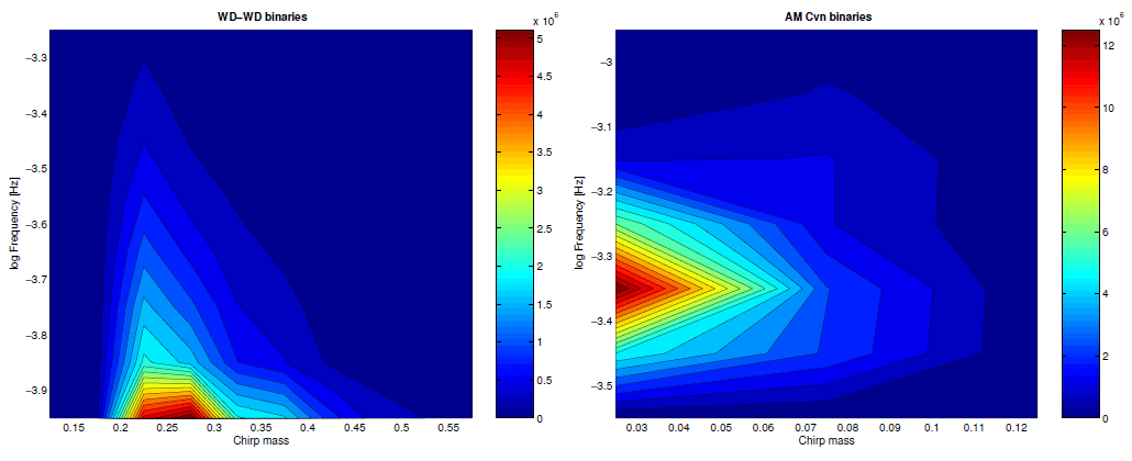
 of 1 and 5 [408]. Semidetached WD binaries contribute to the peak between
 and
and  . Image reproduced with permission from [518*], copyright by ESO.
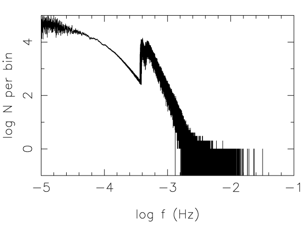
 and
and  . Image reproduced with permission
from
. Image reproduced with permission
from 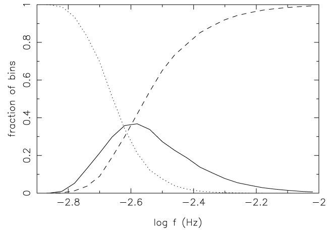
In the model discussed, the systems are distributed randomly in the Galactic disk according to
where
 [664] and
  . The Sun is located at
  and
and  .
Then it is possible to compute the strain amplitude for each system. The power spectrum of the signal from
the population of binaries as it would be detected by a gravitational wave detector, may be simulated by
computation of the distribution of binaries over
.
Then it is possible to compute the strain amplitude for each system. The power spectrum of the signal from
the population of binaries as it would be detected by a gravitational wave detector, may be simulated by
computation of the distribution of binaries over  wide bins, with
  being the total integration
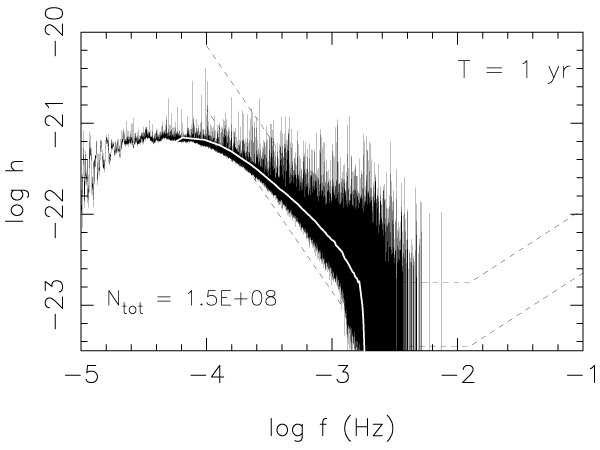
time. Figure 32* shows the resulting confusion limited foreground signal. In Figure 33* the number of
systems per bin is plotted. The assumed integration time is
being the total integration
time. Figure 32* shows the resulting confusion limited foreground signal. In Figure 33* the number of
systems per bin is plotted. The assumed integration time is  . Semidetached WD binaries, which
are less numerous than their detached cousins and have lower strain amplitude, dominate the number of
systems per bin in the frequency interval
. Semidetached WD binaries, which
are less numerous than their detached cousins and have lower strain amplitude, dominate the number of
systems per bin in the frequency interval  producing a peak there, see also
Figure 33*.
producing a peak there, see also
Figure 33*.
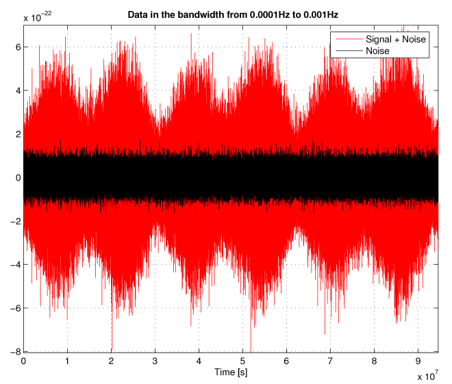
Results presented below may be, to some extent, considered as an illustration of the signal detected by a space-born detector, since they are model-dependent and “LISA-oriented”, but they show, at least qualitatively, the features of the signal detected by any space-based GW antenna.
Figure 32* shows that there are many systems with a signal amplitude much higher than the
average in the bins with  , suggesting that even in the frequency range seized by the
confusion noise some systems can be detectable above the noise level. The latter will affect
the ability to detect extra-galactic massive black-hole binaries (Figure 2*) and to derive their
parameters.
, suggesting that even in the frequency range seized by the
confusion noise some systems can be detectable above the noise level. The latter will affect
the ability to detect extra-galactic massive black-hole binaries (Figure 2*) and to derive their
parameters.
Population synthesis also shows that the notion of a unique “confusion limit” is an artefact of the
assumption of a continuous distribution of systems over their parameters. For a discrete population of
sources it appears that for a given integration time there is actually a range of frequencies where there are
both empty resolution bins and bins containing more than one system (see Figure 34*). For this
“statistical” notion of  , Nelemans et al. [518*] get the first bin containing exactly one system at
 , while up to
  there are bins containing more than one system.
Other authors find similar, but slightly more conservative limits on
there are bins containing more than one system.
Other authors find similar, but slightly more conservative limits on  :
:  [864],
  [828],
 [661].
Nelemans et al. [518*] also noted the following point. Previous studies of GW emission from the
AM CVn systems have found that they hardly contribute to the GW foreground, despite that at
 they outnumber the detached DDs. This happens because at these
  their chirp
mass
their chirp
mass  is much smaller than that of a typical detached system. However, it was overlooked before that
at higher frequencies, where the number of AM CVn systems is much smaller, their
is much smaller than that of a typical detached system. However, it was overlooked before that
at higher frequencies, where the number of AM CVn systems is much smaller, their  is similar to that
of the detached systems from which they descend. This is also confirmed by the latest studies of GW
foreground by Nissanke et al., see Figure 36*.
is similar to that
of the detached systems from which they descend. This is also confirmed by the latest studies of GW
foreground by Nissanke et al., see Figure 36*.
In [518*, 519*] the following objects were considered as resolved: single source per frequency bin with
signal-to-instrument noise ratio (SNR)  for sources that can be resolved above the confusion limit
  or SNR
  for systems with
  that are detectable above the noise level. This resulted in
approximately equal numbers of resolvable detached double degenerates and interacting double degenerates
— about 11 000 objects of every kind.
that are detectable above the noise level. This resulted in
approximately equal numbers of resolvable detached double degenerates and interacting double degenerates
— about 11 000 objects of every kind.
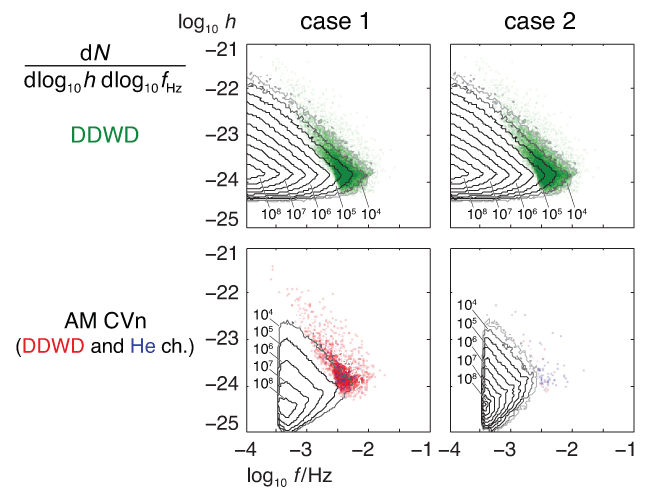
However, the above-mentioned criterion for resolution may be oversimplified. A more rigorous approach implies detection using an iterative identify-and-subtract process, where the signal-to-noise ratio of a source is evaluated with respect to noise from both the instrument and the partially-subtracted foreground [763, 531*]. This procedure was applied by Nissanke et al. [531*] to the same sample of binaries as in [518*, 519*], for both “optimistic”(Case 1 below) and “pessimistic” (Case 2) scenarios (see Sections 7 and 9) with different efficiency of the formation of double degenerates.
 and frequency
  for
close detached WD (top) and AM CVn stars (bottom) in Case 1 and Case 2. Green dots denote
individually-detected WD binary systems (for one year of observation with the 5-Mkm detector); red
dots – AM CVn systems from the WD binary channel and blue dots – AM CVn systems from the
He star channel. Image reproduced with permission from [531*], copyright by AAS.
for
close detached WD (top) and AM CVn stars (bottom) in Case 1 and Case 2. Green dots denote
individually-detected WD binary systems (for one year of observation with the 5-Mkm detector); red
dots – AM CVn systems from the WD binary channel and blue dots – AM CVn systems from the
He star channel. Image reproduced with permission from [531*], copyright by AAS.Figure 36* shows the frequency-space density and GW foreground of WD and AM CVn binary systems for these two scenarios, as computed in [531*]. Qualitatively the results are in good agreement with [518*, 519*], despite the fact that the predicted number of systems is lower by a factor of five.
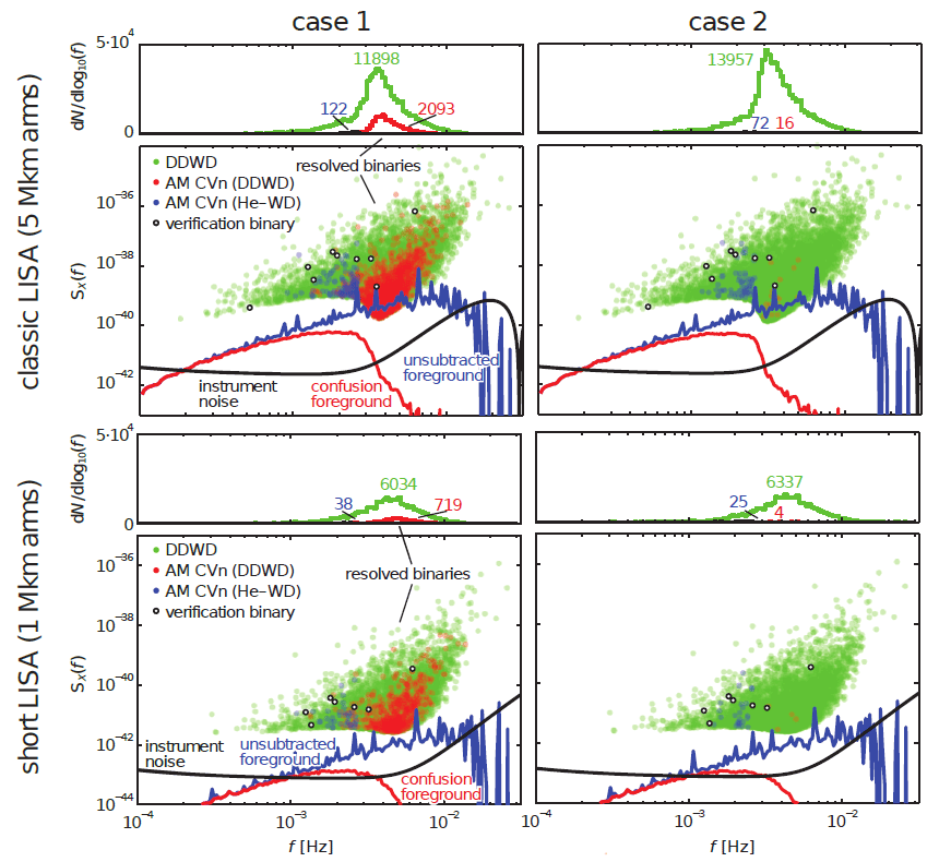
The frequency-space density and GW foreground of DD and AM CVn systems for two scenarios are shown in Figure 37* and appropriate numbers of systems are presented in Table 9.
 , one interferometric observable, and one year of observation, with
approximate scalings as a function of
, one interferometric observable, and one year of observation, with
approximate scalings as a function of  [531].
|
DD
|
AM CVn (DD)
|
AM CVn (He–WD)
|
|
| case 1 | 11, 898 × (ρeff∕5)−1.4 | 2, 093 × (ρ eff∕5)−1.8 | 122 × (ρ eff∕5)−2.8 |
| case 2 | 13, 957 × (ρeff∕5)−1.4 | 16 × (ρ eff∕5)−1.7 | 72 × (ρ eff∕5)−2.9 |
| case 1 | 6, 034 × (ρeff∕5)−1.2 | 719 × (ρ eff∕5)−1.4 | 38 × (ρ eff∕5)−2.6 |
| case 2 | 6, 337 × (ρeff∕5)−1.2 | 4 × (ρ eff∕5)−1.4 | 25 × (ρ eff∕5)−2.2 |
The estimates were made for two assumed arm-lengths of the detector. The number of detected sources
and the level of residual confusion foreground may be scaled by power laws of a single “effective-SNR
parameter”  , where
  is the detection threshold,
  is the
time of observations, and
is the
time of observations, and  is the number of Time-Delayed Interferometry observables (TDI – a
specific method to properly time-shift and linearly combine independent Doppler measurements, that is
necessary in the case of unequal arm-lengths of the detector [150];
is the number of Time-Delayed Interferometry observables (TDI – a
specific method to properly time-shift and linearly combine independent Doppler measurements, that is
necessary in the case of unequal arm-lengths of the detector [150];  for a two-arms configuration
of the detector).
for a two-arms configuration
of the detector).
For the LISA-like configuration, the number of detected DDs is comparable to earlier estimates for the
“optimistic” case of [518*, 519*]:  11 000. The number of AM CVn stars that was comparable to the
number of DDs, now strongly drops due to a higher required SNR defined with respect to both instrument
and confusion noise and the usage of interferometric observables instead of the strain. For a 1 Mkm
detector, the effect of changing detection criterion is much more profound – by a factor of two to four. The
more rigorous detection criterion changes the number of AM CVn stars more than the number
of DD, since the former have smaller chirp mass and strain amplitudes. Thus, the conclusion
of early studies on the dominance of detached DD in the GW foreground formation remains
valid.
11 000. The number of AM CVn stars that was comparable to the
number of DDs, now strongly drops due to a higher required SNR defined with respect to both instrument
and confusion noise and the usage of interferometric observables instead of the strain. For a 1 Mkm
detector, the effect of changing detection criterion is much more profound – by a factor of two to four. The
more rigorous detection criterion changes the number of AM CVn stars more than the number
of DD, since the former have smaller chirp mass and strain amplitudes. Thus, the conclusion
of early studies on the dominance of detached DD in the GW foreground formation remains
valid.
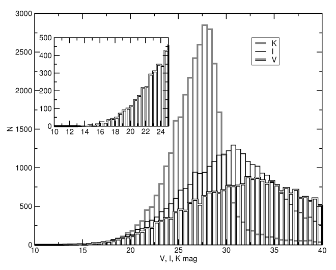
 -band, the
black line the distribution in the
-band, the
black line the distribution in the  -band and the grey histogram the distribution in the
  -band.
Galactic absorption is taken into account. The insert shows the bright-end tail of the
-band.
Galactic absorption is taken into account. The insert shows the bright-end tail of the  -band
distribution. Image reproduced with permission from [509], copyright by IOP.
-band
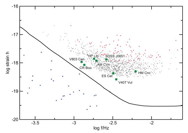
distribution. Image reproduced with permission from [509], copyright by IOP. Peculiarly enough, as Figure 35* shows, the AM CVn-type systems appear, in fact, dominant among the
“verification binaries” for LISA/eLISA: binaries that are well known from electromagnetic observations and
whose radiation is estimated to be sufficiently strong to be detected; see the list of 30 promising candidates
in [744] and references therein. The perspectives and strategy of discovering additional verification
binaries were discussed by Littenberg et al. [433*], who used as an input catalog the model
from [519*] with minor modifications. It was shown in [433] that for the “optimistic” scenario of
the formation of AM CVn stars,  arm-length configuration (full LISA), a 63%
confidence interval of the sky-location posterior distribution area on the celestial sphere and
limiting stellar magnitude of the sample
arm-length configuration (full LISA), a 63%
confidence interval of the sky-location posterior distribution area on the celestial sphere and
limiting stellar magnitude of the sample  the number of candidate double-degenerate
verification binaries is
the number of candidate double-degenerate
verification binaries is  560. For the “pessimistic” scenario, short arm-length (
 ,
similar to eLISA),
,
similar to eLISA),  ,
,  this number reduces to 9. If an additional detection
requirement of being eclipsing is applied, these numbers are reduced by a factor of
this number reduces to 9. If an additional detection
requirement of being eclipsing is applied, these numbers are reduced by a factor of  3. The
conclusion is that the chance for discovering new “verification binaries” is associated with the
next generation of ground-based telescopes, like the 38-m European Extremely Large Telescope
(E-ELT),34 the 30-m US telescope
(TMT),35 the James Webb
Space Telescope (JWST).36
The ESA GAIA mission will also be very helpful in localization of the sources. Resolved LISA sources are
expected to be most numerous in the
3. The
conclusion is that the chance for discovering new “verification binaries” is associated with the
next generation of ground-based telescopes, like the 38-m European Extremely Large Telescope
(E-ELT),34 the 30-m US telescope
(TMT),35 the James Webb
Space Telescope (JWST).36
The ESA GAIA mission will also be very helpful in localization of the sources. Resolved LISA sources are
expected to be most numerous in the  -band, and a significant fraction of them will have
  (Figure 38*), within reach of the future facilities, whilst current instruments are mostly limited by
 [509].
The most severe “astronomical” problems concerning “verification binaries” are their distances, which for most systems are only estimates, and poorly constrained component masses. Some features of “verification binaries” and prospects of detection of new objects in wide-field surveys are also discussed in [358].
The issue of “verification binaries” is related to the problem of detection of GWR sources in electromagnetic waves which is discussed in the next Section 11.
 |
 |
 |
Living Rev. Relativity, 17 (2014), 3, doi:10.12942/lrr-2014-3, URL (accessed <date>): http://www.livingreviews.org/lrr-2014-3.
 This work is licensed under a Creative Commons License.
© The author(s), except where otherwise noted.
This work is licensed under a Creative Commons License.
© The author(s), except where otherwise noted.